> For the complete documentation index, see [llms.txt](https://osh.fducslg.com/notes/llms.txt). Markdown versions of documentation pages are available by appending `.md` to page URLs; this page is available as [Markdown](https://osh.fducslg.com/notes/database-systems/05-files-and-indices.md).
# Files and Indices
\[TOC]
## Files
File is a collection of pages, each containing a collection of records.

Many alternative file organizations exists, each is good for some situations, and not so good in others.
* Heap Files have no particular order among the records.
They are suitable when the typical access is a file scan retrieving all records.
They are also feasible for inserting records.
* Sorted Files: pages and records within pages are ordered by some condition
Best for retrieval (of a range of records) in some order
They are also feasible for finding and manipulating some records.
* Index File Organizations
Special data structure that has the fastest retrieval in some order
### Heap Files
Simplest file structure, contains records in no particular order. As file grows and shrinks, disk pages are allocated and de-allocated. Fastest for **inserts** compared to other alternatives

### Sorted Files
Similar structure like heap files (pages and records), but pages and records are ordered.
Fast for range queries, but hard for maintenance( each insert potentially reshuffles records )

***
DBMS model the cost of all operations
The cost is typically expressed in **the number of page accesses** (or disk **I/O operations** - to bring data from disk to memory)
1 page access (on disk) == 1 I/O (used interchangeably)
## Index
Sometimes, we want to retrieve records by specifying the values in one or more fields.
An index is a data structure built on top of data pages used for efficient search. The index is built over specific fields called **search key fields.**
**Any** subset of the fields of a relation can be the search key for an index on the relation.
An index contains a collection of **data entries**, and supports efficient retrieval pf **data records** matching a given search condition.

## Index Classification
Classification based on various factors:
* Clustered vs. Unclustered
* Primary vs. Secondary
* Single Key vs. Composite
* Indexing technique: Tree-based, hash-based, other
### Clustered vs. Unclustered
If **order of data records** is the same as the **order of index data entrie**s, then the index is called clustered index. Otherwise is unclustered.
A data file can have a clustered index on at most **one search key combination**. (i.e. we cannot have multiple clustered indexes over a single table)
Cost of retrieving data records through index varies greatly based on whether index is clustered. (cheaper for clustered)
Clustering indexes are more expensive to maintain (require file reorganization), but are really efficient for **range search.**
Approximated cost of retrieving records found in range scan:
1. Clustered: cost $$\approx$$ $#$ of pages in data file with matching records
2. Unclustered: cost$$\approx$$ $#$ of matching index data entries (data records)
### Primary vs. Secondary Index
* **Primary** index includes the table’s **primary key**
* **Secondary** is any other index
Properties:
* Primary index never contains duplicates
* Secondary index may contain duplicates
### Composite Search Keys
An index can be built over a combination of search keys.
Data entries in index sorted by search keys.
Examples:
1. Index on $$\$$
2. Index on $$\$$
### Hash-based Index
Hash-based index
* Represents index as a collection of buckets. Hash function maps the search key to the corresponding bucket.
$$h(r.search\_key) =$$ bucket in which record $$r$$ belongs
* Good for **equality-based** selections
## Index: Implemented with B+ Tree
### Properties
* **Order:** The order of a B+ tree is represented by `d`. Each node, excluding the root, is required to have between `d` and `2d` entries under normal conditions without deletions. However, leaf nodes may have fewer than `d` entries following data deletions.
* **Fanout:** The fanout of a B+ tree refers to the maximum number of children a node can have, which is `2d+1`.
* **Leaf Nodes:** All leaf nodes in a B+ tree are positioned at the same depth and maintain between `d` and `2d` entries, ensuring they are at least half full.
* **Height:** The height of a B+ tree is defined by the number of edges needed to traverse from the root node to any leaf node.
### Insertion
1. Find the leaf node $$L$$ in which you will insert your value. Add the key and the record to the leaf node in order.
2. If $$L$$ overflows
1. Split into $$L\_1$$ and $$L\_2$$. Keep $$d$$ entries in $$L\_1$$ (this means $$d+1$$ entries will go in $$L\_2$$).
2. If $$L$$ was a leaf node, **COPY** $$L\_2$$’s first entry into the parent. If $$L$$ was not a leaf node, **MOVE** $$L\_2$$’s first entry into the parent.
3. Adjust pointers.
3. If the parent overflows, then recurse on it by doing step 2 on the parent.
### Deletion
Just find the appropriate leaf and delete the unwanted value from that leaf. In practice we get *way* more insertions than deletions so something will quickly replace whatever we delete.
### Store Records
**Alternative 1: By Value**
The leaf pages contain the records themselves.
This alternative is clustered by default.
**Limitation**: Cannot support multiple indexes built on the same file (Since the records are ordered by points in the figure below).
**Alternative 2: By Reference**
The leafs contain (Key, RecordID) pairs where the RecordID is \[PageNum, RecordNum].
**Alternative 3: By List of References**
The leaf pages hold lists of pointers to the corresponding records.
### Counting IOs
1. Read the appropriate root-to-leaf path.
2. Read the appropriate data page(s). If we need to read multiple pages, we will allot a read IO for each page. In addition, we account for clustering for Alt. 2 or 3 (see below.)
3. Write data page, if you want to modify it. Again, if we want to do a write that spans multiple data pages, we will need to allot a write IO for each page.
4. Update index page(s).
### Bulk Loading
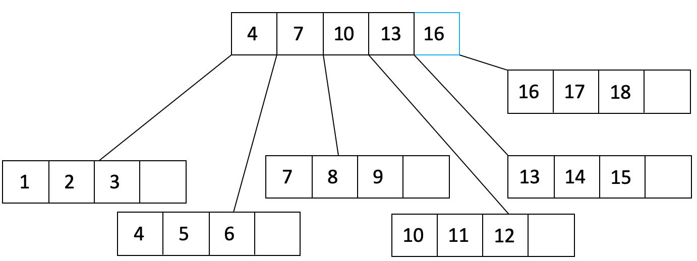
Construct a B+ tree from scratch without having to traverse the tree each time we want to insert something new.
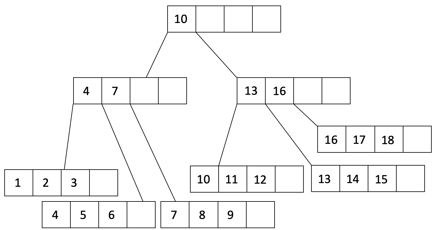
In the following figure, the order is 2 and the fill factor is $$\frac{3}{4}$$
After some adjustments: